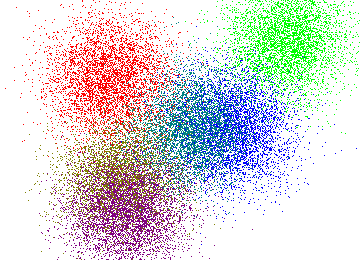
Clustering is one of the main vechicles of machine learning and data analysis. In this post I will describe how to make three very popular sequential clustering algorithms (k-means, single-linkage clustering and correlation clustering) work for big data. The first two algorithms can be used for clustering a collection of feature vectors in \(d\)-dimensional Euclidean space (like the two-dimensional set of points on the picture below, while they also work for high-dimensional data). The last one can be used for arbitrary objects as long as for any pair of them one can define some measure of similarity.
Besides optimizing different objective functions these algorithms also give qualitatively different types of clusterings. K-means produces a set of exactly k clusters. Single-linkage clustering gives a hierarchical partitioning of the data, which one can zoom into at different levels and get any desired number of clusters. Finally, in correlation clustering the number of clusters is not known in advance and is chosen by the algorithm itself in order to optimize a certain objective function.
All algorithms described in this post use the model for massively parallel computation that I described before.
K-Means
First algorithm is a parallel version of an approximation algorithm for K-Means, one of the most widely used clustering methods. Given a set of vectors \(v_1, \dots, v_n \in \mathbb R^d\) the goal of k-means is to partition them into \(k\) clusters \(S_1, \dots, S_k\) such that the following objective is minimized: $$\sum_{i = 1}^k \sum_{j \in S_i} ||v_j - \mu_i||^2,$$ where \(\mu_i = \frac{1}{|S_i|}\sum_{j \in S_i} v_j\) is the center (or mean) of the \(i\)-th cluster and \(||\cdot||\) is the Euclidean distance. Intuitively, the goal is to pick a partitioning that minimizes the total variance. K-means works great for partitioning into compact groups like those on the picure below.
K-means++ and K-means||
An algorithm for k-means, which gives a clustering of cost within a multiplicative factor \(O(\log k)\) of the optimum was given by Arthur and Vassilvitskii. Here is their algorithm called K-means++:
- Let \(\mathcal C = \{v_i\}\) for a random vector \(v_i\).
- Repeat \(k - 1\) times: let \(\mathcal C = \mathcal C \cup \{u\}\), where \(u\) is a random vector from the probability distribution assigning to each \(v_i\)probability density $$p_i(\mathcal C) = \frac{d(v_i, \mathcal C)^2}{\sum_{i} d(v_i, \mathcal C)^2},$$ where \(d(u,\mathcal C) =\min_{x \in \mathcal C}{||u - x||}.\)
However, K-means++ is sequential and takes at least \(k\) rounds. A parallel version of it called K-means|| is due to Bahmani, Moseley, Vattani, Kumar and Vassilvitskii:
- Let \(\mathcal C = \{v_i\}\) for a random vector \(v_i\)
- Let \(\psi = \sum_{i} d(v_i, \mathcal C)\) be the initial cost of the clustering.
- Repeat \(O(\log \psi)\) times:
- Let \(\mathcal C'\) be a set of \(O(k)\) points each sampled independently from the distribution assigning to \(v_i\) probability \(p_i(\mathcal C)\) defined above.
- \(\mathcal C = \mathcal C \cup \mathcal C'\)
- For each \(x \in \mathcal C\), let \(w_x\) be the number of points belonging to this center
- Recluster the weighted points in \(\mathcal C\) into \(k\) clusters using K-means++
The potential \(\psi\) can be shown to be at most \(poly(n)\) by discretizing the space by a grid with step size \(1/poly(n)\), and moving each point to the closest grid point, which only perturbs the cost of the solution by a negligible factor. Thus we have \(\log \psi = O(\log n)\). The final reclustering can be performed in one round, assuming that \(O(k \log n)\) weighted centers fit on a single machine. Thus, the total number of rounds in the algorithm above is \(O(\log n)\). It can be shown that the solution produced by this algorithm has cost within \(O(\log k)\) of the optimum. For more details I would recommend to see either the original paper or these slides from our reading group by Steven Wu.
Single-Linkage Clustering
Single-linkage clustering is another standard technique in data analysis and information retrieval. It can be used to produce a hierarhical clustering of the data (see also Chapter 17 in the Information Retrieval book by Manning, Raghavan and Schutze and Chapter 7.2 in the Mining of Massive Datasets book by Leskovec, Rajaraman and Ullman).
For two clusters \(S_i\) and \(S_j\) the single linkage distance is defined as: $$D(S_i, S_j) = \min_{v \in S_i, u \in S_j} d(v,u),$$ In general, \(d(\cdot, \cdot)\) can be an arbitrary distance function, but for points in Euclidean space it is most natural to use \(d(v,u) = ||v - u||\). The goal of single linkage clustering in Euclidean space is to partition the set of vectors \(v_1, \dots, v_n \in \mathbb R^d\) into clusters \(S_1, \dots, S_k\) such that the following objective is maximized: $$\min_{i < j} D(S_i, S_j) = \min_{i < j} \min_{v \in S_i, u \in S_j} ||v - u||.$$
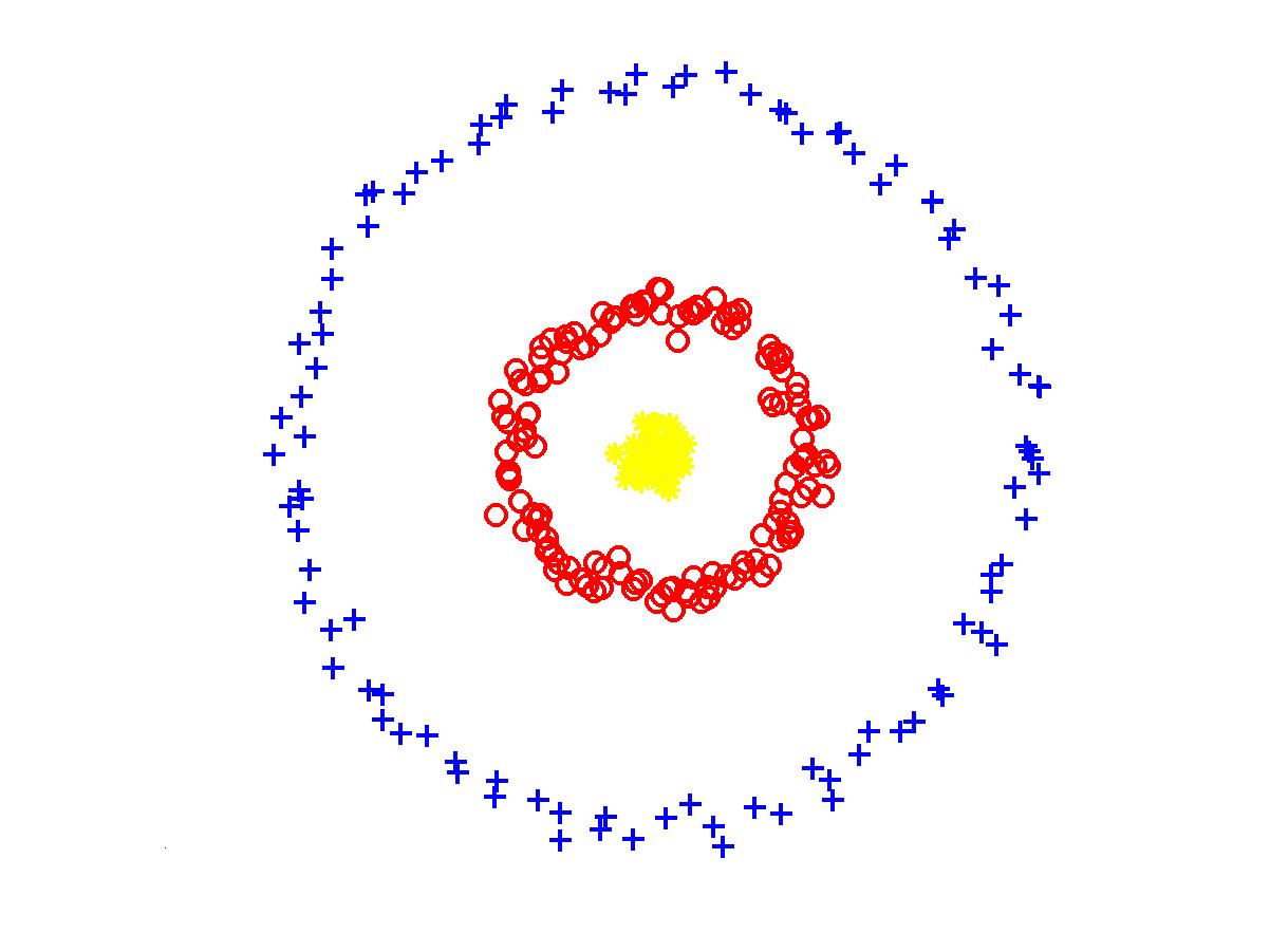
In fact, it is easy to see that the set of clusters \(S_1, \dots S_k\), which maximizes the objective above can be obtained by constructing a Euclidean Minimum Spanning Tree and picking \(S_i\)'s as connected components of this tree obtained after removing \(k - 1\) of its longest edges. Thus, single-linkage clustering works best for finding clusters defined by the connectivity structure. In particular, it can be used to solve the following example which is hard for K-means because points in the cluster are far from their average. This example is typically given as a motivation for using spectral clustering, which I don't discuss in this post, but it can be also addressed using single-linkage:
As expalined above, Euclidean Minimum Spanning Tree can be used to produce hierarchical Single-Linkage Clustering for any number of clusters. However, it is not known how to efficiently compute an exact such tree in small number of rounds of MapReduce. For any constant dimension \(d\) Euclidean Minimum Spanning Tree of cost within \((1 + \epsilon)\)-factor of optimum can be computed in constant number of rounds of MapReduce. This is a result from our joint paper with Alexandr Andoni, Krzysztof Onak and Aleksandar Nikolov, which appeared in STOC 2014. I will cover this algorithm in one of the future posts, but for now you can use the slides of my talk about it.
Correlation Clustering
Correlation clustering can be used to cluster an arbitrary collection of \(n\) objects, so for this type of clustering it is not necessary that they can be represented by vectors in Euclidean space. The only requirement is that for every pair of objects \(i\) and \(j\) it should be possible to compare them directly and obtain a measure of dissimilarity \(w(i,j) \in [0,1]\). Here \(w(i,j) = 0\) means that the objects are exactly the same, while \(w(i,j) = 1\) means that they are completely different and the values in between correspond to different degrees of dissimilarity.
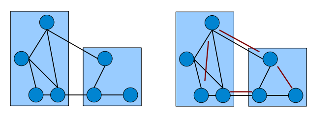
The objective of correlation clustering is to minimize the total cost of mistakes incurred by the clustering. For a set of clusters \(\mathcal C = \mathcal C_1, \dots, \mathcal C_k\) let the indicator function \(x(i,j)\) be defined as \(x(i,j) = 0\) if \(i\) and \(j\) are in the same cluster and \(x(i,j) = 1\) otherwise. The total cost of the clustering is expressed as a function of w's and x's as follows: $$\sum_{i < j \colon x(i,j) = 0} w(i,j) + \sum_{i < j \colon x(i,j) = 1} 1 - w(i,j).$$ Note that the number of clusters is not fixed and the algorithm has to choose it in order to optimize the objective function above. The picture below (courtesy Edo Liberty) uses edges to represent similar pairs (\(w(i,j) = 0\)) and non-edges for dissimilar pairs (\(w(i,j) = 1\)). On the right pairs misclassifed by the clustering are shown in red, so the overall cost of such clustering is equal to 4.
There exist many approximation algorithms for correlation clustering. In particular, using linear programming one can obtain a clustering of total cost within a multiplicative factor 2.5 of the optimum. This is a result of Ailon, Charikar and Newman. Moreover, if the weight function \(w\) satisfies triangle inequalities then the approximation of their algorithm becomes 2. The linear programming relaxation for this problem is naturally formulated using triangle inequalities: $$\text{Minimize: }\sum_{i<j} w(i,j)\cdot (1 - x(i,j)) + (1 - w(i,j)) \cdot x(i,j)$$ $$x(i,j) \le x(i,k) + x(k,j), \text{ } \forall i, j, k$$ $$0 \le x(i,j) \le 1$$ Note that for \(x(i,j) \in \{0,1\}\) this program exactly captures the correlation clustering problem. Recently in joint work with Shuchi Chawla, Konstantin Makarychev and Tselil Schramm we have shown that there is a rounding scheme that achieves approximations 2.06 and 1.5 for these two cases, which is very close to the integrality gaps of this linear progarmming relaxation (2 and 1.2 for the general and triangle inequality cases respectively).
While the linear programming approach is hard to implement in MapReduce there is a very simple combinatorial algorithm due to Ailon, Charikar and Newman, which achieves a 3-approximation in general and a 2-approximation if the weights satisfy triangle inequalities. First, define two sets of edges \(E^+ = \{(i,j) | w(i,j) < 1/2\}\) and \(E^- = \{(i,j) | w(i,j) \ge 1/2\}\). This means that we will treat pairs with dissimilarity below \(1/2\) as similar and those with dissimilarity at least \(1/2\) as dissimilar. Now a set of clusters, which achieves the approximations stated above can be constructed using the following algorithm:
- Pick a random object \(i\)
- Set \(\mathcal C = \{i\}\), \(V' = \emptyset\)
- For all \(j \neq i\):
- If \((i,j) \in E^+\) then add \(j\) to \(\mathcal C\)
- Else if \((i,j) \in E^-\) then add \(j\) to \(V'\)
- Let \(G'\) be the subgraph induce by \(V'\)
- Return clustering consisting of \(\mathcal C\) together with the set of clusters produced by this algorithm applied recursively to \(V'\)
The analysis of approximation achieved by this algorithm cleverly uses linear programming duality. However, this approach is very sequential in nature and might take \(O(n)\) rounds of MapReduce if implemented as is. Recently there has been a paper in KDD 2014 by Chierichetti, Dalvi and Kumar who show that a substantially modified version of the pivoting algorithm above achieves a \((3 + \epsilon)\)-approximation in \(O\left(\frac{\log n \log \Delta^+}{\epsilon}\right)\) rounds, where \(\Delta^+\) is the maximum degree in the graph induced by \(E^+\).